Which Macro Factors explain the price of Bitcoin?

Disclaimer: This is not financial advice and does not constitute a solicitation to buy or sell any financial instrument and/or virtual currency such as Bitcoin. You should always do your own research and consult a professional financial advisor before investing. The views herein represent the private views of the author only and not necessarily of his employer.
The Debate
There is an ongoing debate in the crypto community about which macro factors have been influencing the price of Bitcoin recently. Some would say that Bitcoin has been highly-correlated with equity prices and that it’s just another ‘risk-on’ trade like any other. Obviously, Bitcoin is one of most volatile assets out there, so there’s some truth to that. In fact, Bitcoin sold off during the Covid-shock in Februrary/March 2020 just like the S&P 500 did and has been recovering in a similar fashion as well.

Only this week, Bitcoin has apparently started to decouple from the overall equity market mostly driven by the news that PayPal is going to allow users to buy & sell cryptocurrencies on their platform as well.
At the same time, many pundits are convinced that monetary policy has been the only game in town for Bitcoin, i.e. the ‘money printer go Brrr’ argument. In fact, there appears to be a tight correlation this year between Bitcoin and the stock of negative yielding debt as well.

Statistically speaking, both correlations can hold at the same time since both equities and Bitcoin could be influenced by a third unobserved factor. In the coming section, I will try to elucidate on how to measure macro factors that explain the majority of variations in financial markets and how these macro factors are able to explain the price of Bitcoin.
What ‘explains’ financial markets in general?
I will present a statistical method called ‘Principal Component Analysis’ (PCA) which is able to reduce the complexity of financial markets to a hand full of prevalent factors that are able to explain the majority of financial market price variations. To my knowledge, this approach to financial markets has been pioneered at Goldman Sachs but I have seen similar approaches at other research houses. The power of PCA basically lies in the fact that these factors are relatively-uncorrelated to one another which allows us to ‘filter out’ the common variations that exist among financial market prices and focus on truly distinctive factors.
In order to do so, I will use 26 different daily closing prices from various asset classes such as Equities, Corporate Credit, Sovereign Bonds, FX & Commodities. All the time series in this article have been sourced either from Yahoo! Finance, Investing.com or the Fed of St. Louis Database (FRED). I employ a 1-year rolling standard deviation (z-score) on these market prices in order to ensure stationarity and comparability among the variables.
The computations are performed with R and the prcomp function of the stats package. The results show that the first 4 principal components are already able to explain approximately 2/3 of the variations of these 26 financial market variables. So we reduced the whole dataset from 26 to 4 variables but reduced explanatory power only by a third. We could calculate even more factors but we stick with these first 4 since the marginal contribution to the overall explanatory power decreases with every additional factor.
Now comes the hard part: How do we classify these different principal components into macro factors?
One of the drawbacks of PCA is that there is an element of interpretation in how to classify the different principal components. Most of the time, a researcher is also forced to change the algebraic sign of the factor in order to make it better interpretable (so-called ‘factor rotation’). The following tables show the partial R² (i.e. the respective amount of variation explained) of the first 4 prinicipal components (PC 1 — PC 4) and the most important market variables, respectively:

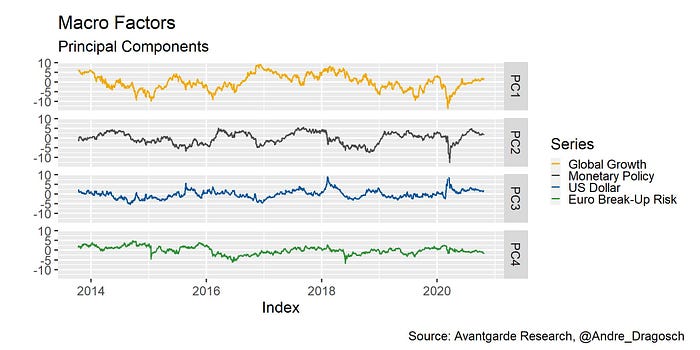
The first principal component (PC1) appears to be correlated with all kinds of ‘growth-sensitive’ assets such as US Cyclicals vs Defensives equity sector. In fact, this macro factor exhibits high covariation with leading macro indicators like the ISM Manufacturing New Export Orders which is why I simply call this factor ‘Global Growth’.

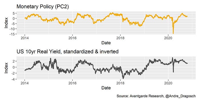
The second principal component (PC2) appears to be correlated with assets that are usually sensitive to changes in (US) monetary policy such as EM Sovereign Bonds or Gold which is why I simply call this factor ‘Monetary Policy’. This factor also shows high covariation with the change in real US bond yields — generally a good proxy for US monetary policy.

The third principal component (PC3) mainly appears to be correlated to exchange rates like the EUR/USD or the Dollar Index (DXY) which is why I simply call this factor ‘US Dollar’.

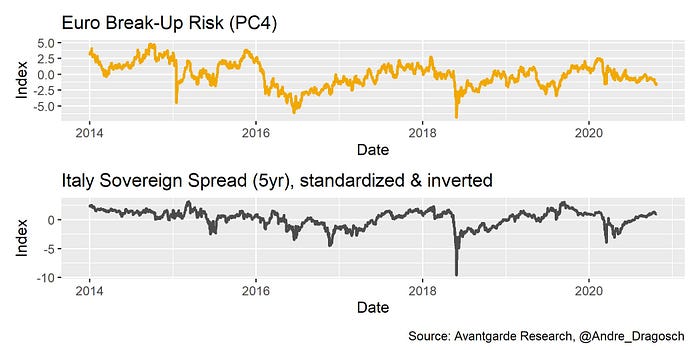
The fourth and last principal component (PC4) appears to be correlated to variables that can signal risks associated with a break-up of the European Monetary Union such as Italian Sovereign Spreads or the CHF/GBP exchange rate which is why I simply call this factor ‘Euro Break-Up Risk’.

Putting it all together
Now that we have computed the different macro factors, we can finally compare the variations of them with the price of Bitcoin.

Before we do so, it is important to note that correlations are not static but dynamic, i.e. change over time. Researchers often speak of ‘regimes’ to seize on this notion of time-varying correlations among variables.
Bitcoin is no different. The subsequent analysis will show differing correlations in different periods of time which is also consistent with observations in the crypto community that Bitcoin sometimes ‘behaves’ more like a Tech stock (rallyes with rising risk appetite) and sometimes more like a safe haven asset such as Gold (rallyes with falling risk appetite).
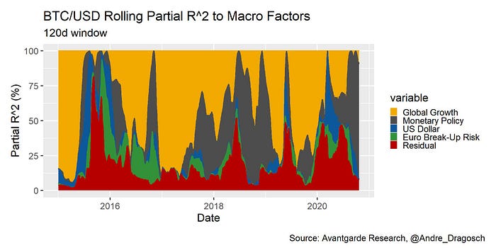
First of all, let’s have a look at the so-called rolling partial R² of the abovementioned macro factors with respect to the price of Bitcoin. In this analysis, the price of Bitcoin refers to the BTC/USD exchange rate provided by CoinMetrics.io. Partial R² represents the percentage of variation in the price of Bitcoin explained by a macro factor in isolation. Rolling simply means that we are looking at a rolling time window (in this case 120 business days). This is what we get:

As mentioned above, the amount of variation in the price of Bitcoin by a single macro factor changes over time and is anything but static. There are also periods when most of the variation in the price of Bitcoin cannot be explained by these macro factors (e.g. end of 2015) which is shown with the red area in Figure 6 (‘Residual’). These are probably periods when Bitcoin was more sensitive to crypto-specific factors but we don’t know exactly. Nonetheless, these 4 macro factors are already able to explain approximately 82% of Bitcoin price variations in the period from Jan 2015 until Oct 2020.
The first and second principal components (‘Global Growth’ (PC1) and ‘Monetary Policy’ (PC2)) historically explain the majority of variations from Jan 2015 until Oct 2020 with 45% and 24%, respectively. So Bitcoin is primarily an asset which rather appears to be sensitive to gyrations in global growth prospects than to changes in monetary policy.
However, since the beginning of 2020, the proportion of Bitcoin price variations explained by the monetary policy factor (PC2) has significantly increased and currently stands at 82% as well while other factors are comparatively insignificant. In other words, expansionary monetary policy has indeed been the most dominant macro factor for Bitcoin this year.
Summing up, these are key findings of this analysis:
These 4 macro factors are already able to explain approximately 82% of Bitcoin price variations in the period from Jan 2015 until Oct 2020.
Bitcoin is primarily an asset which rather appears to be sensitive to gyrations in global growth prospects than to changes in monetary policy.
Expansionary monetary policy has indeed been the most dominant macro factor for Bitcoin in 2020.
About the author of Avantgarde Digital Research Blog:
André Dragosch has been working for almost 10 years in the German financial industry, mostly in Portfoliomanagement and Investment Research. He is currently working as a cross asset analyst and investment strategist at one of the largest German asset managers in Frankfurt. He is currently doing a PhD as well in financial history at the University of Southampton, UK, where amongst others Prof. Richard Werner has supervised his work. He is been a private crypto investor since 2014. He is a married father who loves playing drums, running and travelling.
